Using other compositional differentiation methods in scCODA
While the scCODA package is mainly aimed at providing an implementation and interface of the scCODA model (Büttner, Ostner et al., 2021), the module sccoda.models.other_models contains a variety of wrappers for other compositional differentiation methods that can be used with scCODA’s data handling pipeline.
The available methods are:
A fully Bayesian Dirichlet-Multinomial model without spike-and-slab priors.
The SCDC model (Cao et al., 2019)
A (non-compositional) Poisson regression model
A model using the centered logratio (CLR) transform together with a generalized linear model
A (non-compositional) t-test
A CLR transform together with a t-test
The ALDEx2 model for compositional differentiation in microbial data (Fernandes et al., 2014)
An additive logratio (ALR) transform of the data paired with a t-test
An ALR transform of the data paired with a Wilcoxon rank-sum test
The ANCOM model for compositional differentiation in microbial data (Mandal et al., 2015)
The Bias-corrected ANCOM model for compositional differentiation in microbial data (Lin, Peddada, 2020]
A Dirichlet regression approach (Maier, 2014)
Beta-Binomial modeling via corncob (Martin e al., 2019)
Note: Some methods (SCDC, ALDEx2, Dirichlet Regression, ANCOMBC, Beta-Binomial) require an R environment with the according packages installed
NOTE: If you want to run this tutorial, make sure to have `scikit-bio <https://github.com/biocore/scikit-bio>`__ installed. It is not automatically included when installing via pip.
This tutorial aims at showcasing the use of some of these methods.
Setup and data handling
We use the salmonella infection data from Haber et al., 2017.
[1]:
# Setup
import warnings
warnings.filterwarnings("ignore")

import pandas as pd
import patsy as pt
import numpy as np

from sccoda.model import other_models as om
from sccoda.util import cell_composition_data as dat
from sccoda.util import data_visualization as viz
[2]:
# Get some data (Salmonella infection from Haber et al.)
cell_counts = pd.read_csv("../data/haber_counts.csv")

# Convert data to anndata object
data_all = dat.from_pandas(cell_counts, covariate_columns=["Mouse"])

# Extract condition from mouse name and add it as an extra column to the covariates
data_all.obs["Condition"] = data_all.obs["Mouse"].str.replace(r"_[0-9]", "")

# Select control and salmonella data
data_salm = data_all[data_all.obs["Condition"].isin(["Control", "Salm"])]
print(data_salm)
View of AnnData object with n_obs × n_vars = 6 × 8
    obs: 'Mouse', 'Condition'
[3]:
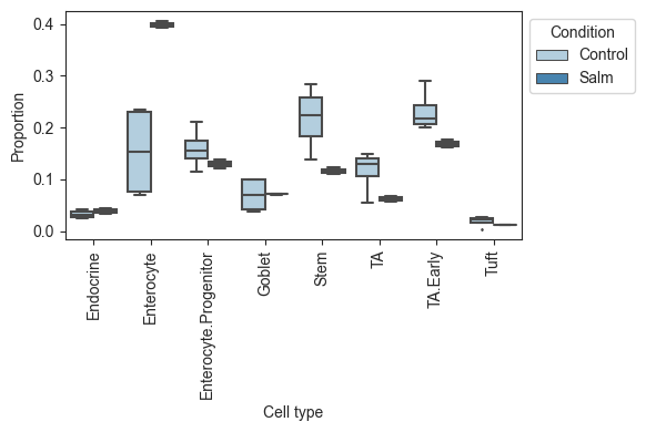
viz.boxplots(data_salm, feature_name="Condition")
[3]:
<AxesSubplot:xlabel='Cell type', ylabel='Proportion'>
The ancom model
Using the ancom model (Mandal et al., 2015) with scCODA is straightforward. We use the implementation in scikit-bio and also its output format:
The column “Reject null hypothesis” shows the columns that change significantly according to ancom
[4]:
ancom_model = om.AncomModel(data_salm, covariate_column="Condition")
ancom_model.fit_model()
print(ancom_model.ancom_out)
Trying to set attribute `.X` of view, copying.
(                       W  Reject null hypothesis
Endocrine              0                   False
Enterocyte             0                   False
Enterocyte.Progenitor  0                   False
Goblet                 0                   False
Stem                   0                   False
TA                     0                   False
TA.Early               0                   False
Tuft                   0                   False, Percentile              0.0     25.0    50.0    75.0    100.0  0.0     25.0   \
Group                 Control Control Control Control Control   Salm    Salm
Endocrine                 5.0   20.75    31.0   38.25    45.0   32.0   33.25
Enterocyte               46.0   55.75    78.5  128.75   221.0  332.0  342.25
Enterocyte.Progenitor    23.0  107.75   162.0  190.50   198.0  113.0  113.75
Goblet                   20.0   32.00    36.0   58.00   124.0   59.0   61.00
Stem                     50.0  110.75   185.0  241.75   250.0   90.0   96.75
TA                       11.0   96.50   127.5  136.25   155.0   47.0   51.50
TA.Early                 40.0  153.25   193.5  238.25   365.0  132.0  141.00
Tuft                      4.0    4.75    11.5   21.75    33.0   10.0   10.50

Percentile             50.0    75.0   100.0
Group                   Salm    Salm   Salm
Endocrine               34.5   35.75   37.0
Enterocyte             352.5  362.75  373.0
Enterocyte.Progenitor  114.5  115.25  116.0
Goblet                  63.0   65.00   67.0
Stem                   103.5  110.25  117.0
TA                      56.0   60.50   65.0
TA.Early               150.0  159.00  168.0
Tuft                    11.0   11.50   12.0  )
The ALDEx2 model
The ALDEx2 model (Fernandes et al., 2014) requires an R installation with the ALDEx2 package available. The paths r_home and r_path must point to the installation folder and the R executable of your R version.
The result columns show the p-values of various tests (see the documentation of ALDEx2 for details)
[5]:
r_home = "/Library/Frameworks/R.framework/Resources"
r_path = "/Library/Frameworks/R.framework/Resources/bin/R"
[6]:
aldex2_model = om.ALDEx2Model(data_salm, covariate_column="Condition")
aldex2_model.fit_model(r_home=r_home, r_path=r_path)
print(aldex2_model.result)
R[write to console]: operating in serial mode

R[write to console]: computing center with all features
      we.ep    we.eBH     wi.ep    wi.eBH
1  0.385566  0.520241  0.519792  0.670258
2  0.055019  0.190518  0.133333  0.419444
3  0.554758  0.649357  0.742708  0.839306
4  0.549451  0.649280  0.890104  0.910625
5  0.045055  0.170609  0.146875  0.427778
6  0.211257  0.380195  0.436458  0.651677
7  0.165477  0.311701  0.277604  0.509593
8  0.644732  0.715048  0.594792  0.750084
The SCDC model
For using the SCDC model (Cao et al., 2019), an R environment with the package scdney (available on github) is required.
Using the model is similar to the other ones, the “p.values” column shows significances:
[7]:
scdc_model = om.scdney_model(data_salm, covariate_column="Condition")
result, _ = scdc_model.analyze(r_home=r_home, r_path=r_path)
print(result)
R[write to console]: ── Attaching packages ────────────────────────────────────────── scdney 0.2.0 ──

R[write to console]: ✔ scMerge    1.10.0     ✔ scClust    0.3.0
✔ scClassify 1.6.0      ✔ Cepo       1.0.0
✔ CiteFuse   1.6.0      ✔ scHOT      1.6.0
✔ scDC       0.1.0

R[write to console]: ── Attaching packages ─────────────────────────────────────── tidyverse 1.3.1 ──

R[write to console]: ✔ ggplot2 3.3.5     ✔ purrr   0.3.4
✔ tibble  3.1.6     ✔ dplyr   1.0.7
✔ tidyr   1.1.4     ✔ stringr 1.4.0
✔ readr   2.1.0     ✔ forcats 0.5.1

R[write to console]: ── Conflicts ────────────────────────────────────────── tidyverse_conflicts() ──
✖ stringr::boundary() masks graph::boundary()
✖ dplyr::collapse()   masks IRanges::collapse()
✖ dplyr::combine()    masks Biobase::combine(), BiocGenerics::combine()
✖ dplyr::desc()       masks IRanges::desc()
✖ tidyr::expand()     masks S4Vectors::expand()
✖ dplyr::filter()     masks stats::filter()
✖ dplyr::first()      masks S4Vectors::first()
✖ dplyr::lag()        masks stats::lag()
✖ ggplot2::Position() masks BiocGenerics::Position(), base::Position()
✖ purrr::reduce()     masks IRanges::reduce()
✖ dplyr::rename()     masks S4Vectors::rename()
✖ dplyr::select()     masks AnnotationDbi::select(), MASS::select()
✖ dplyr::slice()      masks IRanges::slice()
[1] "Calculating sample proportion..."
[1] "Calculating bootstrap proportion..."
[1] "Calculating BCa ..."
[1] "Calculating z0 ..."
[1] "Calculating acc ..."
[1] "fitting GLM... 10"
[1] "fitting GLM... 20"
[1] "fitting GLM... 30"
[1] "fitting GLM... 40"
[1] "fitting GLM... 50"
[1] "fitting GLM... 60"
[1] "fitting GLM... 70"
[1] "fitting GLM... 80"
[1] "fitting GLM... 90"
[1] "fitting GLM... 100"
                                              term  estimate  std.error  \
0                                      (Intercept)  3.340425   0.130826
1                         cellTypescell_Enterocyte  1.318058   0.151683
2              cellTypescell_Enterocyte.Progenitor  1.573899   0.145437
3                             cellTypescell_Goblet  0.643168   0.167195
4                               cellTypescell_Stem  1.779897   0.138821
5                                 cellTypescell_TA  1.324436   0.145850
6                           cellTypescell_TA.Early  1.944167   0.143707
7                               cellTypescell_Tuft -0.654497   0.225239
8                                       condCond_1  0.178457   0.216167
9              cellTypescell_Enterocyte:condCond_1  1.026114   0.234573
10  cellTypescell_Enterocyte.Progenitor:condCond_1 -0.346556   0.250467
11                 cellTypescell_Goblet:condCond_1 -0.033054   0.262500
12                   cellTypescell_Stem:condCond_1 -0.659463   0.239814
13                     cellTypescell_TA:condCond_1 -0.808348   0.257086
14               cellTypescell_TA.Early:condCond_1 -0.450709   0.241865
15                   cellTypescell_Tuft:condCond_1 -0.527277   0.429530

    statistic         df       p.value
0   25.533339  22.224333  0.000000e+00
1    8.689552  20.875604  2.240259e-08
2   10.821880  21.667775  3.348521e-10
3    3.846807  20.668018  9.586014e-04
4   12.821524  23.109362  5.442757e-12
5    9.080787  22.648182  5.234775e-09
6   13.528677  20.981438  7.842393e-12
7   -2.905783  21.966284  8.204102e-03
8    0.825554  21.753691  4.180192e-01
9    4.374399  21.402135  2.554530e-04
10  -1.383638  20.350230  1.814600e-01
11  -0.125920  22.708496  9.009037e-01
12  -2.749898  22.420741  1.156695e-02
13  -3.144273  22.698956  4.592254e-03
14  -1.863476  20.683645  7.665614e-02
15  -1.227567  20.908642  2.332512e-01
The simple Dirichlet-Multinomial model
Using the simple Dirichlet model is similar to using the scCODA model. Only HMC sampling is available for inference.
Significantly changing are all cell types where 0 is not included in the high density interval (HDI)
[10]:
K = data_salm.X.shape[1]
formula = "Condition"

cell_types = data_salm.var.index.to_list()

# Get count data
data_matrix = data_salm.X.astype("float32")

# Build covariate matrix from R-like formula
covariate_matrix = pt.dmatrix(formula, data_salm.obs)
covariate_names = covariate_matrix.design_info.column_names[1:]
covariate_matrix = covariate_matrix[:, 1:]

# Init model. Baseline index is always the last cell type
mod = om.SimpleModel(covariate_matrix=np.array(covariate_matrix), data_matrix=data_matrix,
                     cell_types=cell_types, covariate_names=covariate_names, formula=formula,
                     reference_cell_type=4)

# Run HMC sampling
result_simple = mod.sample_hmc()

result_simple.summary_extended()
2021-11-28 19:36:25.016681: W tensorflow/core/grappler/costs/op_level_cost_estimator.cc:689] Error in PredictCost() for the op: op: "Softmax" attr { key: "T" value { type: DT_DOUBLE } } inputs { dtype: DT_DOUBLE shape { unknown_rank: true } } device { type: "CPU" vendor: "GenuineIntel" model: "110" frequency: 2000 num_cores: 8 environment { key: "cpu_instruction_set" value: "AVX SSE, SSE2, SSE3, SSSE3, SSE4.1, SSE4.2" } environment { key: "eigen" value: "3.4.99" } l1_cache_size: 49152 l2_cache_size: 524288 l3_cache_size: 6291456 memory_size: 268435456 } outputs { dtype: DT_DOUBLE shape { unknown_rank: true } }
2021-11-28 19:36:25.038579: W tensorflow/core/grappler/costs/op_level_cost_estimator.cc:689] Error in PredictCost() for the op: op: "Softmax" attr { key: "T" value { type: DT_DOUBLE } } inputs { dtype: DT_DOUBLE shape { unknown_rank: true } } device { type: "CPU" vendor: "GenuineIntel" model: "110" frequency: 2000 num_cores: 8 environment { key: "cpu_instruction_set" value: "AVX SSE, SSE2, SSE3, SSSE3, SSE4.1, SSE4.2" } environment { key: "eigen" value: "3.4.99" } l1_cache_size: 49152 l2_cache_size: 524288 l3_cache_size: 6291456 memory_size: 268435456 } outputs { dtype: DT_DOUBLE shape { unknown_rank: true } }
MCMC sampling finished. (283.799 sec)
Acceptance rate: 69.1%
Compositional Analysis summary (extended):

Data: 6 samples, 8 cell types
Reference index: 4
Formula: Condition

MCMC Sampling: Sampled 20000 chain states (5000 burnin samples) in 283.799 sec. Acceptance rate: 69.1%

Intercepts:
                       Final Parameter  HDI 3%  HDI 97%     SD  \
Cell Type
Endocrine                        1.043   0.307    1.726  0.387
Enterocyte                       2.320   1.723    2.930  0.323
Enterocyte.Progenitor            2.483   1.834    3.075  0.334
Goblet                           1.616   0.924    2.227  0.351
Stem                             2.746   2.179    3.371  0.317
TA                               2.161   1.467    2.807  0.355
TA.Early                         2.849   2.233    3.440  0.324
Tuft                             0.410  -0.382    1.213  0.431

                       Expected Sample
Cell Type
Endocrine                    32.431823
Enterocyte                  116.296171
Enterocyte.Progenitor       136.884860
Goblet                       57.520427
Stem                        178.063484
TA                           99.200211
TA.Early                    197.381842
Tuft                         17.221182


Effects:
                                         Final Parameter  HDI 3%  HDI 97%  \
Covariate         Cell Type
Condition[T.Salm] Endocrine                     0.529575  -0.323    1.414
                  Enterocyte                    1.608336   1.096    2.167
                  Enterocyte.Progenitor         0.329774  -0.243    0.936
                  Goblet                        0.575193  -0.140    1.276
                  Stem                               NaN   0.000    0.000
                  TA                           -0.056400  -0.733    0.606
                  TA.Early                      0.230121  -0.316    0.751
                  Tuft                          0.133425  -0.972    1.171

                                            SD  Inclusion probability  \
Covariate         Cell Type
Condition[T.Salm] Endocrine              0.463               0.999200
                  Enterocyte             0.283               1.000000
                  Enterocyte.Progenitor  0.311               0.998333
                  Goblet                 0.380               0.999333
                  Stem                   0.000               0.000000
                  TA                     0.356               0.998467
                  TA.Early               0.285               0.998200
                  Tuft                   0.569               0.998800

                                         Expected Sample  log2-fold change
Covariate         Cell Type
Condition[T.Salm] Endocrine                    35.638644          0.136032
                  Enterocyte                  375.850562          1.692356
                  Enterocyte.Progenitor       123.177940         -0.152219
                  Goblet                       66.158172          0.201845
                  Stem                               NaN               NaN
                  TA                           60.670369         -0.709351
                  TA.Early                    160.770249         -0.295989
                  Tuft                         12.734065         -0.435491
Frequentist tests
Frequentist tests can all be used with the same scheme. Here, we use the ALR-transformed t-test as an example. The p.val attribute always contains the p-values of the test for all cell types (except the reference type if using ALR transforms).
[9]:
alr_t_model = om.ALRModel_ttest(data_salm, covariate_column="Condition")
alr_t_model.fit_model(reference_cell_type=4)
print(alr_t_model.p_val)
[0.061904043349529855, 0.016550016833625263, 0.01594225849767037, 0.4157960379583721, 1, 0.2886155729884671, 0.11388003371717678, 0.4785462482431266]