Modeling options and result analysis in scCODA
This tutorial notebook serves as an extension to the general tutorial and presents ways to alternate the model and perform more in-depth result analysis and diagnostics. We will focus on:
Modifications of the model formula and reference cell type to perform different modeling tasks
Inference methods available in scCODA
Advanced interpretation and analysis of results
Alternative differential abundance testing using all references
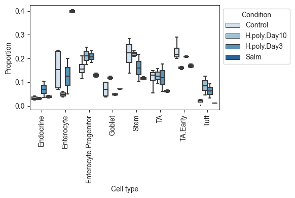
We will again analyze the small intestinal epithelium data of mice from Haber et al., 2017. First, we read in the data and perform the same preprocessing steps as in the general tutorial:
[1]:
# Setup
import warnings
warnings.filterwarnings("ignore")

import pandas as pd
import matplotlib.pyplot as plt
import arviz as az

from sccoda.util import comp_ana as mod
from sccoda.util import cell_composition_data as dat
from sccoda.util import data_visualization as viz
[2]:
# Load data
cell_counts = pd.read_csv("../data/haber_counts.csv")

# Convert data to anndata object
data_all = dat.from_pandas(cell_counts, covariate_columns=["Mouse"])

# Extract condition from mouse name and add it as an extra column to the covariates
data_all.obs["Condition"] = data_all.obs["Mouse"].str.replace(r"_[0-9]", "")
print(f"Entire dataset: {data_all}")

# Select control and salmonella data
data_salm = data_all[data_all.obs["Condition"].isin(["Control", "Salm"])].copy()
print(f"Salmonella dataset: {data_salm}")

viz.boxplots(data_all, feature_name="Condition")
plt.show()
Entire dataset: AnnData object with n_obs × n_vars = 10 × 8
    obs: 'Mouse', 'Condition'
Salmonella dataset: AnnData object with n_obs × n_vars = 6 × 8
    obs: 'Mouse', 'Condition'
Tweaking the model formula and reference cell type
First, we take a closer look at how changing the formula parameter of the scCODA model influences the results. Internally, the formula string is converted into a linear model-like design matrix via patsy, which has a similar syntax to the lm function in the R language.
Multi-level categories
Patsy allows us to automatically handle categorical covariates, even with multiple levels. For example, we can model the effect of all three diseases at once:
[3]:
# model all three diseases at once
model_all = mod.CompositionalAnalysis(data_all, formula="Condition", reference_cell_type="Endocrine")
all_results = model_all.sample_hmc()
all_results.summary()
2021-11-28 19:15:21.670317: I tensorflow/core/platform/cpu_feature_guard.cc:142] This TensorFlow binary is optimized with oneAPI Deep Neural Network Library (oneDNN) to use the following CPU instructions in performance-critical operations:  AVX2 FMA
To enable them in other operations, rebuild TensorFlow with the appropriate compiler flags.
WARNING:tensorflow:From /Users/johannes.ostner/opt/anaconda3/envs/scCODA_3/lib/python3.8/site-packages/tensorflow/python/ops/array_ops.py:5043: calling gather (from tensorflow.python.ops.array_ops) with validate_indices is deprecated and will be removed in a future version.
Instructions for updating:
The `validate_indices` argument has no effect. Indices are always validated on CPU and never validated on GPU.
2021-11-28 19:15:23.943628: I tensorflow/compiler/mlir/mlir_graph_optimization_pass.cc:176] None of the MLIR Optimization Passes are enabled (registered 2)
  0%|          | 0/20000 [00:00<?, ?it/s]2021-11-28 19:15:25.649198: I tensorflow/compiler/xla/service/service.cc:169] XLA service 0x7fd21d1c63a0 initialized for platform Host (this does not guarantee that XLA will be used). Devices:
2021-11-28 19:15:25.649348: I tensorflow/compiler/xla/service/service.cc:177]   StreamExecutor device (0): Host, Default Version
2021-11-28 19:15:28.022894: I tensorflow/compiler/jit/xla_compilation_cache.cc:337] Compiled cluster using XLA!  This line is logged at most once for the lifetime of the process.
100%|██████████| 20000/20000 [01:38<00:00, 203.36it/s]
MCMC sampling finished. (123.099 sec)
Acceptance rate: 78.2%
Compositional Analysis summary:

Data: 10 samples, 8 cell types
Reference index: 0
Formula: Condition

Intercepts:
                       Final Parameter  Expected Sample
Cell Type
Endocrine                        0.986        46.634633
Enterocyte                       1.905       116.902874
Enterocyte.Progenitor            2.348       182.061302
Goblet                           1.474        75.970374
Stem                             2.427       197.027528
TA                               1.878       113.788726
TA.Early                         2.534       219.278684
Tuft                             0.626        32.535879


Effects:
                                                 Final Parameter  \
Covariate                 Cell Type
Condition[T.H.poly.Day10] Endocrine                     0.000000
                          Enterocyte                    0.000000
                          Enterocyte.Progenitor         0.000000
                          Goblet                        0.000000
                          Stem                          0.000000
                          TA                            0.000000
                          TA.Early                      0.000000
                          Tuft                          0.000000
Condition[T.H.poly.Day3]  Endocrine                     0.000000
                          Enterocyte                    0.000000
                          Enterocyte.Progenitor         0.000000
                          Goblet                        0.000000
                          Stem                          0.000000
                          TA                            0.000000
                          TA.Early                      0.000000
                          Tuft                          0.000000
Condition[T.Salm]         Endocrine                     0.000000
                          Enterocyte                    1.554932
                          Enterocyte.Progenitor         0.000000
                          Goblet                        0.000000
                          Stem                          0.000000
                          TA                            0.000000
                          TA.Early                      0.000000
                          Tuft                          0.000000

                                                 Expected Sample  \
Covariate                 Cell Type
Condition[T.H.poly.Day10] Endocrine                    46.634633
                          Enterocyte                  116.902874
                          Enterocyte.Progenitor       182.061302
                          Goblet                       75.970374
                          Stem                        197.027528
                          TA                          113.788726
                          TA.Early                    219.278684
                          Tuft                         32.535879
Condition[T.H.poly.Day3]  Endocrine                    46.634633
                          Enterocyte                  116.902874
                          Enterocyte.Progenitor       182.061302
                          Goblet                       75.970374
                          Stem                        197.027528
                          TA                          113.788726
                          TA.Early                    219.278684
                          Tuft                         32.535879
Condition[T.Salm]         Endocrine                    32.304092
                          Enterocyte                  383.418044
                          Enterocyte.Progenitor       126.114963
                          Goblet                       52.625137
                          Stem                        136.482158
                          TA                           78.822138
                          TA.Early                    151.895669
                          Tuft                         22.537800

                                                 log2-fold change
Covariate                 Cell Type
Condition[T.H.poly.Day10] Endocrine                      0.000000
                          Enterocyte                     0.000000
                          Enterocyte.Progenitor          0.000000
                          Goblet                         0.000000
                          Stem                           0.000000
                          TA                             0.000000
                          TA.Early                       0.000000
                          Tuft                           0.000000
Condition[T.H.poly.Day3]  Endocrine                      0.000000
                          Enterocyte                     0.000000
                          Enterocyte.Progenitor          0.000000
                          Goblet                         0.000000
                          Stem                           0.000000
                          TA                             0.000000
                          TA.Early                       0.000000
                          Tuft                           0.000000
Condition[T.Salm]         Endocrine                     -0.529685
                          Enterocyte                     1.713608
                          Enterocyte.Progenitor         -0.529685
                          Goblet                        -0.529685
                          Stem                          -0.529685
                          TA                            -0.529685
                          TA.Early                      -0.529685
                          Tuft                          -0.529685
Different reference levels
Per default, categorical variables are encoded via full-rank treatment coding. Hereby, the value of the first sample in the dataset is used as the default (control) category. We can select the default level by changing the model formula to "C(<CovariateName>, Treatment('<ReferenceLevelName>'))":
For example, we can switch the salmonella model to test diseased versus healthy samples, which switches the sign of the only credible effect (Enterocytes).
[4]:
# Set salmonella infection as "default" category

model_salm_switch_cond = mod.CompositionalAnalysis(data_salm, formula="C(Condition, Treatment('Salm'))", reference_cell_type="Goblet")
switch_results = model_salm_switch_cond.sample_hmc()
switch_results.summary()
100%|██████████| 20000/20000 [01:02<00:00, 317.86it/s]
MCMC sampling finished. (82.254 sec)
Acceptance rate: 49.8%
Compositional Analysis summary:

Data: 6 samples, 8 cell types
Reference index: 3
Formula: C(Condition, Treatment('Salm'))

Intercepts:
                       Final Parameter  Expected Sample
Cell Type
Endocrine                        1.269        28.559849
Enterocyte                       3.708       327.340808
Enterocyte.Progenitor            2.566       104.480647
Goblet                           1.777        47.465439
Stem                             2.615       109.727702
TA                               2.048        62.240247
TA.Early                         2.877       142.594061
Tuft                             0.450        12.591247


Effects:
                                                                  Final Parameter  \
Covariate                                  Cell Type
C(Condition, Treatment('Salm'))[T.Control] Endocrine                     0.000000
                                           Enterocyte                   -1.365487
                                           Enterocyte.Progenitor         0.000000
                                           Goblet                        0.000000
                                           Stem                          0.000000
                                           TA                            0.000000
                                           TA.Early                      0.000000
                                           Tuft                          0.000000

                                                                  Expected Sample  \
Covariate                                  Cell Type
C(Condition, Treatment('Salm'))[T.Control] Endocrine                    40.336384
                                           Enterocyte                  118.009650
                                           Enterocyte.Progenitor       147.562807
                                           Goblet                       67.037616
                                           Stem                        154.973463
                                           TA                           87.904755
                                           TA.Early                    201.392129
                                           Tuft                         17.783195

                                                                  log2-fold change
Covariate                                  Cell Type
C(Condition, Treatment('Salm'))[T.Control] Endocrine                      0.498093
                                           Enterocyte                    -1.471889
                                           Enterocyte.Progenitor          0.498093
                                           Goblet                         0.498093
                                           Stem                           0.498093
                                           TA                             0.498093
                                           TA.Early                       0.498093
                                           Tuft                           0.498093
Switching the reference cell type
Compositional analysis generally does not allow statements on absolute abundance changes, but only in relation to a reference category, which is assumed to be unchanged in absolute abundance. The reference cell type fixes this category in scCODA. Thus, an interpretation of scCODA’s effects should always be formulated like:
“Using cell type xy as a reference, cell types (a, b, c) were found to credibly change in abundance”
Switching the reference cell type might thus produce different results. For example, if we choose a different cell type as the reference (such as Enterocytes in the salmonella infection data), scCODA can find other credible effects on the other cell types.
[13]:
model_salm_ref = mod.CompositionalAnalysis(data_salm, formula="Condition", reference_cell_type="Enterocyte")
reference_results = model_salm_ref.sample_hmc()
reference_results.summary()
100%|██████████| 20000/20000 [01:02<00:00, 321.43it/s]
MCMC sampling finished. (80.035 sec)
Acceptance rate: 54.2%
Compositional Analysis summary:

Data: 6 samples, 8 cell types
Reference index: 1
Formula: Condition

Intercepts:
                       Final Parameter  Expected Sample
Cell Type
Endocrine                        0.563        34.927176
Enterocyte                       2.088       160.495387
Enterocyte.Progenitor            1.870       129.058424
Goblet                           1.100        59.755737
Stem                             2.095       161.622796
TA                               1.475        86.944084
TA.Early                         2.220       183.142621
Tuft                            -0.043        19.053774


Effects:
                                         Final Parameter  Expected Sample  \
Covariate         Cell Type
Condition[T.Salm] Endocrine                          0.0        34.927176
                  Enterocyte                         0.0       160.495387
                  Enterocyte.Progenitor              0.0       129.058424
                  Goblet                             0.0        59.755737
                  Stem                               0.0       161.622796
                  TA                                 0.0        86.944084
                  TA.Early                           0.0       183.142621
                  Tuft                               0.0        19.053774

                                         log2-fold change
Covariate         Cell Type
Condition[T.Salm] Endocrine                           0.0
                  Enterocyte                          0.0
                  Enterocyte.Progenitor               0.0
                  Goblet                              0.0
                  Stem                                0.0
                  TA                                  0.0
                  TA.Early                            0.0
                  Tuft                                0.0
Inference algorithms in scCODA
Currently, scCODA performs parameter inference via Markov-chain Monte Carlo (MCMC) methods. There are three different MCMC sampling methods available for scCODA:
Hamiltonian Monte Carlo (HMC) sampling:
sample_hmc()HMC sampling with Dual-averaging step size adaptation (Nesterov, 2009):
sample_hmc_da()No-U-Turn sampling (Hoffman and Gelman, 2014):
sample_nuts()
Generally, it is recommended to use the standard HMC sampling. Other methods, such as variational inference, are in consideration.
For all MCMC sampling methods, properties such as the MCMC chain length and the number of burn-in samples are directly adjustable.
Result analysis and diagnostics
The “getting started” tutorial explains how to do interpret the basic output of scCODA. To follow this up, we now take a look at how MCMC diagnostics and more advanced result analysis in scCODA can be performed.
For this section, we again use the model of salmonella infection versus control group, with a reference cell type of Goblet cells.
[6]:
model_salm = mod.CompositionalAnalysis(data_salm, formula="Condition", reference_cell_type="Goblet")
salm_results = model_salm.sample_hmc(num_results=20000)
100%|██████████| 20000/20000 [01:03<00:00, 314.08it/s]
MCMC sampling finished. (80.894 sec)
Acceptance rate: 55.8%
Extended model summary
result.summary_extended() gives us, apart from the properties already explained in the basic tutorial, more information about the posterior inferred by the model. The extended summary also includes some information on the MCMC sampling procedure (chain length, burn-in, acceptance rate, duration).
For both effects and intercepts, we also get the standard deviation (SD) and high density interval endpoints of the posterior density of the generated Markov chain.
The effects summary also includes the spike-and-slab inclusion probability for each effect, i.e. the share of MCMC samples, for which this effect was not set to 0 by the spike-and-slab prior. A threshold on this value serves as the deciding factor whether an effect is considered statistically credible
We can also use the summary tables from summary_extended() as pandas DataFrames to tweak them further. They are also accessible as result.intercept_df and result.effect_df, respectively. Furthermore, the tables a direct result of the summary() function in arviz and support all its functionality. This means that we can, for example, change the credible interval:
[7]:
salm_results.summary_extended(hdi_prob=0.9)
Compositional Analysis summary (extended):

Data: 6 samples, 8 cell types
Reference index: 3
Formula: Condition
Spike-and-slab threshold: 1.000

MCMC Sampling: Sampled 20000 chain states (5000 burnin samples) in 80.894 sec. Acceptance rate: 55.8%

Intercepts:
                       Final Parameter  HDI 5%  HDI 95%     SD  \
Cell Type
Endocrine                        1.105   0.548    1.750  0.369
Enterocyte                       2.330   1.842    2.844  0.312
Enterocyte.Progenitor            2.517   2.055    3.071  0.310
Goblet                           1.749   1.253    2.277  0.316
Stem                             2.710   2.229    3.235  0.306
TA                               2.114   1.576    2.658  0.330
TA.Early                         2.858   2.361    3.341  0.297
Tuft                             0.433  -0.210    1.065  0.394

                       Expected Sample
Cell Type
Endocrine                    34.199308
Enterocyte                  116.420125
Enterocyte.Progenitor       140.359279
Goblet                       65.118287
Stem                        170.239355
TA                           93.803805
TA.Early                    197.394727
Tuft                         17.465114


Effects:
                                         Final Parameter  HDI 5%  HDI 95%  \
Covariate         Cell Type
Condition[T.Salm] Endocrine                     0.000000  -0.432    1.033
                  Enterocyte                    1.347912   0.912    1.768
                  Enterocyte.Progenitor         0.000000  -0.255    0.581
                  Goblet                        0.000000   0.000    0.000
                  Stem                          0.000000  -0.720    0.129
                  TA                            0.000000  -0.789    0.249
                  TA.Early                      0.000000  -0.331    0.422
                  Tuft                          0.000000  -0.772    0.866

                                            SD  Inclusion probability  \
Covariate         Cell Type
Condition[T.Salm] Endocrine              0.348               0.506933
                  Enterocyte             0.265               1.000000
                  Enterocyte.Progenitor  0.158               0.334800
                  Goblet                 0.000               0.000000
                  Stem                   0.214               0.398667
                  TA                     0.247               0.418933
                  TA.Early               0.119               0.267467
                  Tuft                   0.325               0.417733

                                         Expected Sample  log2-fold change
Covariate         Cell Type
Condition[T.Salm] Endocrine                    24.475708         -0.482617
                  Enterocyte                  320.727867          1.462009
                  Enterocyte.Progenitor       100.452112         -0.482617
                  Goblet                       46.603755         -0.482617
                  Stem                        121.836638         -0.482617
                  TA                           67.133362         -0.482617
                  TA.Early                    141.271153         -0.482617
                  Tuft                         12.499406         -0.482617
Diagnostics and plotting
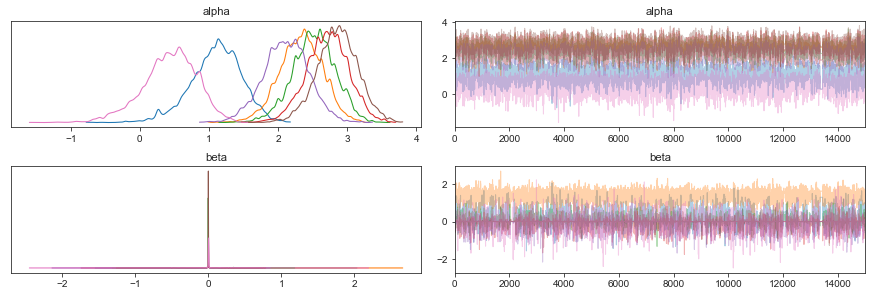
Similarly to the summary dataframes being compatible with arviz, the result class itself is an extension of arviz’s Inference Data class. This means that we can use all its MCMC diagnostic and plotting functionality. As an example, looking at the MCMC trace plots and kernel density estimates, we see that they are indicative of a well sampled MCMC chain:
Note: Due to the spike-and-slab priors, the beta parameters have many values at 0, which looks like a convergence issue, but is actually not.
Caution: Trying to plot a kernel density estimate for an effect on the reference cell type results in an error, since it is constant at 0 for the entire chain. To avoid this, add coords={"cell_type": salm_results.posterior.coords["cell_type_nb"]} as an argument to ``az.plot_trace``, which causes the plots for the reference cell type to be skipped.
[8]:
az.plot_trace(
    salm_results,
    divergences=False,
    var_names=["alpha", "beta"],
    coords={"cell_type": salm_results.posterior.coords["cell_type_nb"]},
)
plt.show()
Using all cell types as reference alternatively to reference selection
scCODA uses a reference cell type that is considered to be unchanged over the experiment to guarantee the unique identifiability of results. If no such cell type is known beforehand, setting reference_cell_type="automatic" will find a suited reference. Alternatively, it is possible to find credible effects on cell types that are mostly independent of the reference. By sequentially running scCODA and selecting each cell type as the reference once, we can then use a majority vote to find the
cell types that were credibly changing more than half of the time.
Below, an example code for this procedure on the Salmonella infection data shows that only Enterocytes were found to be credible more than half of the time. Indeed, they re credibly changing for every reference cell type except themselves. All other cell types were not found to change with any reference.
[9]:
# Run scCODA with each cell type as the reference
cell_types = data_salm.var.index
results_cycle = pd.DataFrame(index=cell_types, columns=["times_credible"]).fillna(0)

for ct in cell_types:
    print(f"Reference: {ct}")

    # Run inference
    model_temp = mod.CompositionalAnalysis(data_salm, formula="Condition", reference_cell_type=ct)
    temp_results = model_temp.sample_hmc(num_results=20000)

    # Select credible effects
    cred_eff = temp_results.credible_effects()
    cred_eff.index = cred_eff.index.droplevel(level=0)

    # add up credible effects
    results_cycle["times_credible"] += cred_eff.astype("int")
Reference: Endocrine
100%|██████████| 20000/20000 [01:03<00:00, 313.42it/s]
WARNING:tensorflow:5 out of the last 5 calls to <function CompositionalModel.sampling.<locals>.sample_mcmc at 0x7fd1ed75e3a0> triggered tf.function retracing. Tracing is expensive and the excessive number of tracings could be due to (1) creating @tf.function repeatedly in a loop, (2) passing tensors with different shapes, (3) passing Python objects instead of tensors. For (1), please define your @tf.function outside of the loop. For (2), @tf.function has experimental_relax_shapes=True option that relaxes argument shapes that can avoid unnecessary retracing. For (3), please refer to https://www.tensorflow.org/guide/function#controlling_retracing and https://www.tensorflow.org/api_docs/python/tf/function for  more details.
MCMC sampling finished. (81.026 sec)
Acceptance rate: 50.1%
Reference: Enterocyte
100%|██████████| 20000/20000 [01:04<00:00, 309.59it/s]
WARNING:tensorflow:6 out of the last 6 calls to <function CompositionalModel.sampling.<locals>.sample_mcmc at 0x7fd1ed75e3a0> triggered tf.function retracing. Tracing is expensive and the excessive number of tracings could be due to (1) creating @tf.function repeatedly in a loop, (2) passing tensors with different shapes, (3) passing Python objects instead of tensors. For (1), please define your @tf.function outside of the loop. For (2), @tf.function has experimental_relax_shapes=True option that relaxes argument shapes that can avoid unnecessary retracing. For (3), please refer to https://www.tensorflow.org/guide/function#controlling_retracing and https://www.tensorflow.org/api_docs/python/tf/function for  more details.
MCMC sampling finished. (85.399 sec)
Acceptance rate: 56.5%
Reference: Enterocyte.Progenitor
100%|██████████| 20000/20000 [01:08<00:00, 291.32it/s]
MCMC sampling finished. (93.835 sec)
Acceptance rate: 60.7%
Reference: Goblet
100%|██████████| 20000/20000 [01:13<00:00, 271.64it/s]
MCMC sampling finished. (90.710 sec)
Acceptance rate: 58.2%
Reference: Stem
100%|██████████| 20000/20000 [01:07<00:00, 295.02it/s]
MCMC sampling finished. (86.994 sec)
Acceptance rate: 51.8%
Reference: TA
100%|██████████| 20000/20000 [01:22<00:00, 242.56it/s]
MCMC sampling finished. (103.528 sec)
Acceptance rate: 53.4%
Reference: TA.Early
100%|██████████| 20000/20000 [01:21<00:00, 244.23it/s]
MCMC sampling finished. (105.065 sec)
Acceptance rate: 54.0%
Reference: Tuft
100%|██████████| 20000/20000 [01:23<00:00, 240.64it/s]
MCMC sampling finished. (104.704 sec)
Acceptance rate: 49.7%
[10]:
# Calculate percentages
results_cycle["pct_credible"] = results_cycle["times_credible"]/len(cell_types)
results_cycle["is_credible"] = results_cycle["pct_credible"] > 0.5
print(results_cycle)
                       times_credible  pct_credible  is_credible
Endocrine                           0         0.000        False
Enterocyte                          7         0.875         True
Enterocyte.Progenitor               0         0.000        False
Goblet                              0         0.000        False
Stem                                0         0.000        False
TA                                  0         0.000        False
TA.Early                            0         0.000        False
Tuft                                0         0.000        False
[10]: