scCODA - Compositional analysis of single-cell data
This notebook serves as a tutorial for using the scCODA package (Büttner, Ostner et al., 2021) to analyze changes in cell composition data.
The package is intended to be used with cell composition from single-cell RNA-seq experiments, however there are no technical restrictions that prevent the use of data from other sources.
The data we use in the following example comes from Haber et al., 2017. It contains samples from the small intestinal epithelium of mice with different conditions.
This tutorial is designed to be executed on a standard computer (any operating system) in a Python environment with scCODA, Jupyter notebook and all their dependencies installed. Running the tutorial takes about 1.5 minutes on a 2020 Apple MacBook Pro (16GB RAM).
[13]:
# Setup
import importlib
import warnings
warnings.filterwarnings("ignore")

import pandas as pd
import pickle as pkl
import matplotlib.pyplot as plt

from sccoda.util import comp_ana as mod
from sccoda.util import cell_composition_data as dat
from sccoda.util import data_visualization as viz

import sccoda.datasets as scd
Data preparation
[14]:
# Load data

cell_counts = scd.haber()

print(cell_counts)
            Mouse  Endocrine  Enterocyte  Enterocyte.Progenitor  Goblet  Stem  \
0       Control_1         36          59                    136      36   239
1       Control_2          5          46                     23      20    50
2       Control_3         45          98                    188     124   250
3       Control_4         26         221                    198      36   131
4  H.poly.Day10_1         42          71                    203     147   271
5  H.poly.Day10_2         40          57                    383     170   321
6   H.poly.Day3_1         52          75                    347      66   323
7   H.poly.Day3_2         65         126                    115      33    65
8          Salm_1         37         332                    113      59    90
9          Salm_2         32         373                    116      67   117

    TA  TA.Early  Tuft
0  125       191    18
1   11        40     5
2  155       365    33
3  130       196     4
4  109       180   146
5  244       256    71
6  263       313    51
7   39       129    59
8   47       132    10
9   65       168    12
Looking at the data, we see that we have 4 control samples, and 3 conditions with 2 samples each. To use the models in scCODA, we first have to convert the data into an anndata object. This can be done easily with the sccoda.util.cell_composition_data module. The resulting object separates our data components: Cell counts are stored in data.X, covariates in data.obs.
[15]:
# Convert data to anndata object
data_all = dat.from_pandas(cell_counts, covariate_columns=["Mouse"])

# Extract condition from mouse name and add it as an extra column to the covariates
data_all.obs["Condition"] = data_all.obs["Mouse"].str.replace(r"_[0-9]", "", regex=True)
print(data_all)
AnnData object with n_obs × n_vars = 10 × 8
    obs: 'Mouse', 'Condition'
AnnData object with n_obs × n_vars = 10 × 8
    obs: 'Mouse', 'Condition'
For our first example, we want to look at how the Salmonella infection influences the cell composition. Therefore, we subset our data.
[16]:
# Select control and salmonella data
data_salm = data_all[data_all.obs["Condition"].isin(["Control", "Salm"])]
print(data_salm.obs)
       Mouse Condition
0  Control_1   Control
1  Control_2   Control
2  Control_3   Control
3  Control_4   Control
8     Salm_1      Salm
9     Salm_2      Salm
       Mouse Condition
0  Control_1   Control
1  Control_2   Control
2  Control_3   Control
3  Control_4   Control
8     Salm_1      Salm
9     Salm_2      Salm
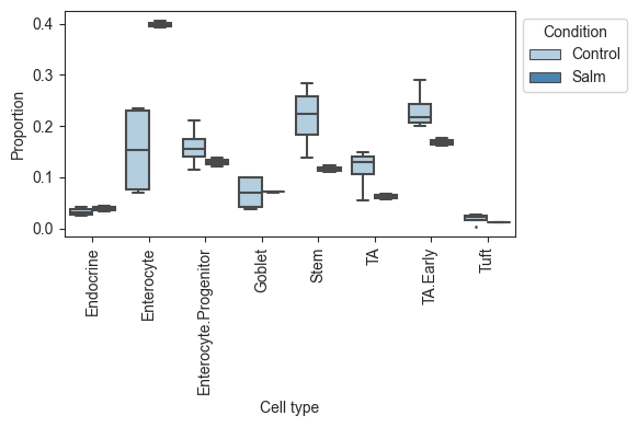
Plotting the data, we can see that there is a large increase of Enterocytes in the infected sampes, while most other cell types slightly decrease. Since scRNA-seq experiments are limited in the number of cells per sample, the count data is compositional, which leads to negative correlations between the cell types. Thus, the slight decreases in many cell types might be fully caused by the increase in Enterocytes.
[17]:
viz.boxplots(data_salm, feature_name="Condition")
plt.show()

Note that the use of anndata in scCODA is different from the use in scRNA-seq pipelines, e.g. scanpy. To convert scanpy objects to a scCODA dataset, have a look at `dat.from_scanpy.
Model setup and inference
We can now create the model and run inference on it. Creating a sccoda.util.comp_ana.CompositionalAnalysis class object sets up the compositional model and prepares everxthing for parameter inference. It needs these informations:
The data object from above.
The
formulaparameter. It specifies how the covariates are used in the model. It can process R-style formulas via the patsy package, e.g.formula="Cov1 + Cov2 + Cov3". Here, we simply use the “Condition” covariate of our datasetThe
reference_cell_typeparameter is used to specify a cell type that is believed to be unchanged by the covariates informula. This is necessary, because compositional analysis must always be performed relative to a reference (See Büttner, Ostner et al., 2021 for a more thorough explanation). If no knowledge about such a cell type exists prior to the analysis, taking a cell type that has a nearly constant relative abundance over all samples is often a good choice. It is also possible to let scCODA find a suited reference cell type by usingreference_cell_type="automatic". Here, we take Goblet cells as the reference.
[18]:
model_salm = mod.CompositionalAnalysis(data_salm, formula="Condition", reference_cell_type="Goblet")
2022-06-27 10:33:10.230757: I tensorflow/core/platform/cpu_feature_guard.cc:151] This TensorFlow binary is optimized with oneAPI Deep Neural Network Library (oneDNN) to use the following CPU instructions in performance-critical operations:  AVX2 AVX512F FMA
To enable them in other operations, rebuild TensorFlow with the appropriate compiler flags.
HMC sampling is then initiated by calling model.sample_hmc(), which produces a sccoda.util.result_classes.CAResult object.
[19]:
# Run MCMC
sim_results = model_salm.sample_hmc()
WARNING:tensorflow:@custom_gradient grad_fn has 'variables' in signature, but no ResourceVariables were used on the forward pass.
WARNING:tensorflow:@custom_gradient grad_fn has 'variables' in signature, but no ResourceVariables were used on the forward pass.
2022-06-27 10:33:13.334993: I tensorflow/compiler/xla/service/service.cc:171] XLA service 0x7f8509aca950 initialized for platform Host (this does not guarantee that XLA will be used). Devices:
2022-06-27 10:33:13.335016: I tensorflow/compiler/xla/service/service.cc:179]   StreamExecutor device (0): Host, Default Version
  0%|          | 0/20000 [00:00<?, ?it/s]2022-06-27 10:33:13.435243: I tensorflow/compiler/mlir/tensorflow/utils/dump_mlir_util.cc:237] disabling MLIR crash reproducer, set env var `MLIR_CRASH_REPRODUCER_DIRECTORY` to enable.
2022-06-27 10:33:14.417583: I tensorflow/compiler/jit/xla_compilation_cache.cc:399] Compiled cluster using XLA!  This line is logged at most once for the lifetime of the process.
100%|██████████| 20000/20000 [00:57<00:00, 348.77it/s]
MCMC sampling finished. (73.009 sec)
Acceptance rate: 55.6%
WARNING:tensorflow:@custom_gradient grad_fn has 'variables' in signature, but no ResourceVariables were used on the forward pass.
WARNING:tensorflow:@custom_gradient grad_fn has 'variables' in signature, but no ResourceVariables were used on the forward pass.
100%|██████████| 20000/20000 [00:51<00:00, 387.96it/s]
MCMC sampling finished. (69.511 sec)
Acceptance rate: 55.4%
Result interpretation
Calling summary() on the results object, we can see the most relevant information for further analysis:
[20]:
sim_results.summary()
Compositional Analysis summary:

Data: 6 samples, 8 cell types
Reference index: 3
Formula: Condition

Intercepts:
                       Final Parameter  Expected Sample
Cell Type
Endocrine                        1.109        34.615689
Enterocyte                       2.325       116.781775
Enterocyte.Progenitor            2.508       140.233238
Goblet                           1.739        64.994784
Stem                             2.693       168.731218
TA                               2.104        93.625897
TA.Early                         2.856       198.602834
Tuft                             0.422        17.414567


Effects:
                                         Final Parameter  Expected Sample  \
Covariate         Cell Type
Condition[T.Salm] Endocrine                     0.000000        24.744607
                  Enterocyte                    1.348671       321.590375
                  Enterocyte.Progenitor         0.000000       100.244037
                  Goblet                        0.000000        46.460736
                  Stem                          0.000000       120.615473
                  TA                            0.000000        66.927342
                  TA.Early                      0.000000       141.968837
                  Tuft                          0.000000        12.448593

                                         log2-fold change
Covariate         Cell Type
Condition[T.Salm] Endocrine                     -0.484312
                  Enterocyte                     1.461409
                  Enterocyte.Progenitor         -0.484312
                  Goblet                        -0.484312
                  Stem                          -0.484312
                  TA                            -0.484312
                  TA.Early                      -0.484312
                  Tuft                          -0.484312
Compositional Analysis summary:

Data: 6 samples, 8 cell types
Reference index: 3
Formula: Condition

Intercepts:
                       Final Parameter  Expected Sample
Cell Type
Endocrine                        1.136        34.655473
Enterocyte                       2.358       117.619596
Enterocyte.Progenitor            2.539       140.957109
Goblet                           1.758        64.551003
Stem                             2.717       168.419124
TA                               2.129        93.546221
TA.Early                         2.877       197.641672
Tuft                             0.459        17.609802


Effects:
                                         Final Parameter  Expected Sample  \
Covariate         Cell Type
Condition[T.Salm] Endocrine                     0.000000        24.773668
                  Enterocyte                    1.343318       322.176411
                  Enterocyte.Progenitor         0.000000       100.764016
                  Goblet                        0.000000        46.144663
                  Stem                          0.000000       120.395398
                  TA                            0.000000        66.872065
                  TA.Early                      0.000000       141.285309
                  Tuft                          0.000000        12.588470

                                         log2-fold change
Covariate         Cell Type
Condition[T.Salm] Endocrine                     -0.484276
                  Enterocyte                     1.453722
                  Enterocyte.Progenitor         -0.484276
                  Goblet                        -0.484276
                  Stem                          -0.484276
                  TA                            -0.484276
                  TA.Early                      -0.484276
                  Tuft                          -0.484276
Model properties
First, the summary shows an overview over the model properties: * Number of samples/cell types * The reference cell type. * The formula used
The model has two types of parameters that are relevant for analysis - intercepts and effects. These can be interpreted like in a standard regression model: Intercepts show how the cell types are distributed without any active covariates, effects show ho the covariates influence the cell types.
Intercepts
The first column of the intercept summary shows the parameters determined by the MCMC inference.
The “Expected sample” column gives some context to the numerical values. If we had a new sample (with no active covariates) with a total number of cells equal to the mean sampling depth of the dataset, then this distribution over the cell types would be most likely.
Effects
For the effect summary, the first column again shows the inferred parameters for all combinations of covariates and cell types. Most important is the distinctions between zero and non-zero entries A value of zero means that no statistically credible effect was detected. For a value other than zero, a credible change was detected. A positive sign indicates an increase, a negative sign a decrease in abundance.
Since the numerical values of the “Final Parameter” column are not straightforward to interpret, the “Expected sample” and “log2-fold change” columns give us an idea on the magnitude of the change. The expected sample is calculated for each covariate separately (covariate value = 1, all other covariates = 0), with the same method as for the intercepts. The log-fold change is then calculated between this expected sample and the expected sample with no active covariates from the intercept section. Since the data is compositional, cell types for which no credible change was detected, can still change in abundance as well, as soon as a credible effect is detected on another cell type due to the sum-to-one constraint. If there are no credible effects for a covariate, its expected sample will be identical to the intercept sample, therefore the log2-fold change is 0.
Interpretation
In the salmonella case, we see only a credible increase of Enterocytes, while all other cell types are unaffected by the disease. The log-fold change of Enterocytes between control and infected samples with the same total cell count lies at about 1.54.
We can also easily filter out all credible effects:
[21]:
print(sim_results.credible_effects())
Covariate          Cell Type
Condition[T.Salm]  Endocrine                False
                   Enterocyte                True
                   Enterocyte.Progenitor    False
                   Goblet                   False
                   Stem                     False
                   TA                       False
                   TA.Early                 False
                   Tuft                     False
Name: Final Parameter, dtype: bool
Adjusting the False discovery rate
scCODA selects credible effects based on their inclusion probability. The cutoff between credible and non-credible effects depends on the desired false discovery rate (FDR). A smaller FDR value will produce more conservative results, but might miss some effects, while a larger FDR value selects more effects at the cost of a larger number of false discoveries.
The desired FDR level can be easily set after inference via sim_results.set_fdr(). Per default, the value is 0.05, but we recommend to increase it if no effects are found at a more conservative level.
In our example, setting a desired FDR of 0.4 reveals effects on Endocrine and Enterocyte cells.
[22]:
sim_results.set_fdr(est_fdr=0.4)
sim_results.summary()
Compositional Analysis summary:

Data: 6 samples, 8 cell types
Reference index: 3
Formula: Condition

Intercepts:
                       Final Parameter  Expected Sample
Cell Type
Endocrine                        1.109        34.615689
Enterocyte                       2.325       116.781775
Enterocyte.Progenitor            2.508       140.233238
Goblet                           1.739        64.994784
Stem                             2.693       168.731218
TA                               2.104        93.625897
TA.Early                         2.856       198.602834
Tuft                             0.422        17.414567


Effects:
                                         Final Parameter  Expected Sample  \
Covariate         Cell Type
Condition[T.Salm] Endocrine                     0.288324        32.681545
                  Enterocyte                    1.348671       318.351944
                  Enterocyte.Progenitor         0.000000        99.234574
                  Goblet                        0.000000        45.992875
                  Stem                          0.000000       119.400870
                  TA                            0.000000        66.253380
                  TA.Early                      0.000000       140.539204
                  Tuft                          0.017884        12.545608

                                         log2-fold change
Covariate         Cell Type
Condition[T.Salm] Endocrine                     -0.082950
                  Enterocyte                     1.446807
                  Enterocyte.Progenitor         -0.498914
                  Goblet                        -0.498914
                  Stem                          -0.498914
                  TA                            -0.498914
                  TA.Early                      -0.498914
                  Tuft                          -0.473112
Compositional Analysis summary:

Data: 6 samples, 8 cell types
Reference index: 3
Formula: Condition

Intercepts:
                       Final Parameter  Expected Sample
Cell Type
Endocrine                        1.136        34.655473
Enterocyte                       2.358       117.619596
Enterocyte.Progenitor            2.539       140.957109
Goblet                           1.758        64.551003
Stem                             2.717       168.419124
TA                               2.129        93.546221
TA.Early                         2.877       197.641672
Tuft                             0.459        17.609802


Effects:
                                         Final Parameter  Expected Sample  \
Covariate         Cell Type
Condition[T.Salm] Endocrine                     0.275744        32.882559
                  Enterocyte                    1.343318       324.574906
                  Enterocyte.Progenitor         0.000000       101.514171
                  Goblet                        0.000000        46.488195
                  Stem                          0.000000       121.291701
                  TA                           -0.235592        53.229151
                  TA.Early                      0.000000       142.337130
                  Tuft                          0.000000        12.682187

                                         log2-fold change
Covariate         Cell Type
Condition[T.Salm] Endocrine                     -0.075761
                  Enterocyte                     1.464423
                  Enterocyte.Progenitor         -0.473575
                  Goblet                        -0.473575
                  Stem                          -0.473575
                  TA                            -0.813463
                  TA.Early                      -0.473575
                  Tuft                          -0.473575
Saving results
The compositional analysis results can be saved as a pickle object via results.save(<path_to_file>).
[23]:
# saving
path = "test"
sim_results.save(path)

# loading
with open(path, "rb") as f:
    sim_results_2 = pkl.load(f)

sim_results_2.summary()
Compositional Analysis summary:

Data: 6 samples, 8 cell types
Reference index: 3
Formula: Condition

Intercepts:
                       Final Parameter  Expected Sample
Cell Type
Endocrine                        1.109        34.615689
Enterocyte                       2.325       116.781775
Enterocyte.Progenitor            2.508       140.233238
Goblet                           1.739        64.994784
Stem                             2.693       168.731218
TA                               2.104        93.625897
TA.Early                         2.856       198.602834
Tuft                             0.422        17.414567


Effects:
                                         Final Parameter  Expected Sample  \
Covariate         Cell Type
Condition[T.Salm] Endocrine                     0.288324        32.681545
                  Enterocyte                    1.348671       318.351944
                  Enterocyte.Progenitor         0.000000        99.234574
                  Goblet                        0.000000        45.992875
                  Stem                          0.000000       119.400870
                  TA                            0.000000        66.253380
                  TA.Early                      0.000000       140.539204
                  Tuft                          0.017884        12.545608

                                         log2-fold change
Covariate         Cell Type
Condition[T.Salm] Endocrine                     -0.082950
                  Enterocyte                     1.446807
                  Enterocyte.Progenitor         -0.498914
                  Goblet                        -0.498914
                  Stem                          -0.498914
                  TA                            -0.498914
                  TA.Early                      -0.498914
                  Tuft                          -0.473112
Compositional Analysis summary:

Data: 6 samples, 8 cell types
Reference index: 3
Formula: Condition

Intercepts:
                       Final Parameter  Expected Sample
Cell Type
Endocrine                        1.136        34.655473
Enterocyte                       2.358       117.619596
Enterocyte.Progenitor            2.539       140.957109
Goblet                           1.758        64.551003
Stem                             2.717       168.419124
TA                               2.129        93.546221
TA.Early                         2.877       197.641672
Tuft                             0.459        17.609802


Effects:
                                         Final Parameter  Expected Sample  \
Covariate         Cell Type
Condition[T.Salm] Endocrine                     0.275744        32.882559
                  Enterocyte                    1.343318       324.574906
                  Enterocyte.Progenitor         0.000000       101.514171
                  Goblet                        0.000000        46.488195
                  Stem                          0.000000       121.291701
                  TA                           -0.235592        53.229151
                  TA.Early                      0.000000       142.337130
                  Tuft                          0.000000        12.682187

                                         log2-fold change
Covariate         Cell Type
Condition[T.Salm] Endocrine                     -0.075761
                  Enterocyte                     1.464423
                  Enterocyte.Progenitor         -0.473575
                  Goblet                        -0.473575
                  Stem                          -0.473575
                  TA                            -0.813463
                  TA.Early                      -0.473575
                  Tuft                          -0.473575
[23]: